This feature allows producing ‘visual explanations’ on how a Convolutional Neural Network (CNN) model based its classification and therefore help interpreting the obtained results. The InceptionTime model is used as an illustration.

Open In Colab

# Run this cell to install the latest version of fastcore shared on github
# !pip install git+https://github.com/fastai/fastai2.git
# Run this cell to install the latest version of fastcore shared on github
# !pip install git+https://github.com/fastai/fastcore.git
# Run this cell to install the latest version of timeseries shared on github
# !pip install git+https://github.com/ai-fast-track/timeseries.git
%reload_ext autoreload
%autoreload 2
%matplotlib inline
from timeseries.all import *
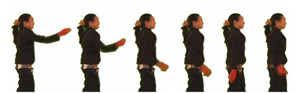
GunPoint Dataset

The dataset was obtained by capturing two actors transiting between yoga poses in front of a green screen. The problem is to discriminate between one actor (male) and another (female). Each image was converted to a one dimensional series by finding the outline and measuring the distance of the outline to the centre.

class CMAP[source]

CMAP()

There are 164 different palettes.

# You can choose any of univariate dataset listed the `data.py` file
dsname =  'GunPoint'
# url = 'http://www.timeseriesclassification.com/Downloads/GunPoint.zip'
path = unzip_data(URLs_TS.UNI_GUN_POINT)
path
Path('/home/farid/.fastai/data/GunPoint')
fname_train = f'{dsname}_TRAIN.arff'
fname_test = f'{dsname}_TEST.arff'
fnames = [path/fname_train, path/fname_test]
fnames
[Path('/home/farid/.fastai/data/GunPoint/GunPoint_TRAIN.arff'),
 Path('/home/farid/.fastai/data/GunPoint/GunPoint_TEST.arff')]
data = TSData.from_arff(fnames)
print(data)
TSData:
 Datasets names (concatenated): ['GunPoint_TRAIN', 'GunPoint_TEST']
 Filenames:                     [Path('/home/farid/.fastai/data/GunPoint/GunPoint_TRAIN.arff'), Path('/home/farid/.fastai/data/GunPoint/GunPoint_TEST.arff')]
 Data shape: (200, 1, 150)
 Targets shape: (200,)
 Nb Samples: 200
 Nb Channels:           1
 Sequence Length: 150
items = data.get_items()
# dls = TSDataLoaders.from_files(fnames=fnames, batch_tfms=batch_tfms, num_workers=0, device=default_device())
dls = TSDataLoaders.from_files(bs=64, fnames=fnames, num_workers=0, device=default_device())
dls.show_batch(max_n=9)

Training Model

# Number of channels (i.e. dimensions in ARFF and TS files jargon)
c_in = get_n_channels(dls.train) # data.n_channels
# Number of classes
c_out= dls.c 
c_in,c_out
(1, 2)
model = inception_time(c_in, c_out).to(device=default_device())
# model
# opt_func = partial(Adam, lr=3e-3, wd=0.01)
#Or use Ranger
def opt_func(p, lr=slice(3e-3)): return Lookahead(RAdam(p, lr=lr, mom=0.95, wd=0.01)) 
#Learner
loss_func = LabelSmoothingCrossEntropy() 
learn = Learner(dls, model, opt_func=opt_func, loss_func=loss_func, metrics=accuracy)
# print(learn.summary())
lr_min, lr_steep = learn.lr_find()
lr_min, lr_steep
(0.017378008365631102, 0.00013182566908653826)
epochs=24; lr_max=1e-3
learn.fit_one_cycle(epochs, lr_max=lr_max)
epoch train_loss valid_loss accuracy time
0 1.313919 0.692904 0.575000 00:00
1 1.248768 0.693099 0.575000 00:00
2 1.141171 0.694189 0.425000 00:00
3 1.070883 0.695346 0.425000 00:00
4 0.944331 0.696796 0.425000 00:00
5 0.842656 0.700287 0.425000 00:00
6 0.757936 0.703399 0.425000 00:00
7 0.685084 0.706720 0.425000 00:00
8 0.626400 0.711806 0.425000 00:00
9 0.579209 0.714237 0.425000 00:00
10 0.539285 0.718178 0.425000 00:00
11 0.505557 0.725727 0.425000 00:00
12 0.476855 0.721790 0.425000 00:00
13 0.452470 0.707657 0.425000 00:00
14 0.431158 0.692659 0.425000 00:00
15 0.412595 0.652262 0.475000 00:00
16 0.396030 0.601834 0.500000 00:00
17 0.381339 0.558574 0.675000 00:00
18 0.368368 0.508540 0.900000 00:00
19 0.356656 0.460236 1.000000 00:00
20 0.346138 0.417405 1.000000 00:00
21 0.336603 0.377413 1.000000 00:00
22 0.328058 0.344103 1.000000 00:00
23 0.320208 0.316467 1.000000 00:00

Graphs

learn.recorder.plot_loss()
# learn.show_results(max_n=9)
interp = ClassificationInterpretation.from_learner(learn)
interp.plot_confusion_matrix()
interp.most_confused()
[]

Heatmap

model = learn.model.eval()
model[5]
SequentialEx(
  (layers): ModuleList(
    (0): InceptionModule(
      (bottleneck): Conv1d(128, 32, kernel_size=(1,), stride=(1,))
      (convs): ModuleList(
        (0): Conv1d(32, 32, kernel_size=(39,), stride=(1,), padding=(19,), bias=False)
        (1): Conv1d(32, 32, kernel_size=(19,), stride=(1,), padding=(9,), bias=False)
        (2): Conv1d(32, 32, kernel_size=(9,), stride=(1,), padding=(4,), bias=False)
      )
      (maxpool_bottleneck): Sequential(
        (0): MaxPool1d(kernel_size=3, stride=1, padding=1, dilation=1, ceil_mode=False)
        (1): Conv1d(128, 32, kernel_size=(1,), stride=(1,), bias=False)
      )
      (bn_relu): Sequential(
        (0): BatchNorm1d(128, eps=1e-05, momentum=0.1, affine=True, track_running_stats=True)
        (1): ReLU()
      )
    )
    (1): Shortcut(
      (act_fn): ReLU(inplace=True)
      (conv): Conv1d(128, 128, kernel_size=(1,), stride=(1,), bias=False)
      (bn): BatchNorm1d(128, eps=1e-05, momentum=0.1, affine=True, track_running_stats=True)
    )
  )
)
model[6]
AdaptiveConcatPool1d(
  (ap): AdaptiveAvgPool1d(output_size=1)
  (mp): AdaptiveMaxPool1d(output_size=1)
)

hooked_backward() function

hooked_backward[source]

hooked_backward(x, y, model, layer)

A function hook to get access to both activation and gradient values of a given model at the layer number layer

Note

Through the notebook, I will be using GunPoint dataset and use its dimensions to illustrate tensors shapes in order to make the code more readable

hook_acts() function

hook_acts[source]

hook_acts(x, y, model, layer)

A hook function to get access to activation values of a given model at the layer number layer

cam_acts[source]

cam_acts(tseries, y, model, layer, reduction='mean', force_scale=True, scale_range=(0, 1))

Compute raw CAM values. reduction : string. One of ['mean', 'median', 'max', 'mean_max']. 'mean_max' corresponds to (mean + max)/2

acts_scaled[source]

acts_scaled(acts, scale_range=(0, 1))

Scale values between [scale_range[0]...scale_range[1]]. By default, it scales acts between 0 and 1

grad_cam_acts[source]

grad_cam_acts(tseries, y, model, layer, reduction='mean', force_scale=True, scale_range=(0, 1))

Compute raw CAM values. reduction : string. One of ['mean', 'median', 'max', 'mean_max']. 'mean_max' corresponds to (mean + max)/2

User defined CAM method

The users can defined their own CAM method and plug it in the show_cam() method. Check out both cam_acts and grad_cam_acts to see how easy you can create your own CAM function

CAM_batch_compute[source]

CAM_batch_compute(b, model, layer=5, func_cam='grad_cam_acts', reduction='mean', force_scale=True, scale_range=(0, 1), linewidths=None, colors=None, antialiaseds=None, linestyles='solid', offsets=None, transOffset=None, norm=None, cmap=None, pickradius=5, zorder=2, facecolors='none')

Compute either CAM for a list (b) of time series tseries .

def _listify(o):
    if o is None: return []
    if isinstance(o, list): return o
    # if is_iter(o): return list(o)
    return [o]

batchify[source]

batchify(dataset, idxs)

Return a list of items for the supplied dataset and idxs

itemize[source]

itemize(batch)

dls.test = dls.train.new(bs=3)
batch = dls.test.one_batch()
# type(batch), len(batch), type(batch[0]), batch
# b = itemize(batch)
# print(b)
# tss, ys = batch
# tss, ys
b = itemize(batch)
# b[0]

get_list_items[source]

get_list_items(dataset, idxs)

Return a list of items for the supplied dataset and idxs

default_device()
device(type='cuda', index=0)

get_batch[source]

get_batch(dataset, idxs)

Return a batch based on list of items from dataset at idxs

idxs = [0,3]
x, y = get_batch(dls.train.dataset, idxs)
x[0].device, x[0]
(device(type='cuda', index=0),
 tensor([[-0.6029, -0.6026, -0.6015, -0.6017, -0.6001, -0.5971, -0.5969, -0.5967,
          -0.5989, -0.5982, -0.5980, -0.5975, -0.5954, -0.5973, -0.5926, -0.5877,
          -0.5867, -0.5845, -0.5827, -0.5834, -0.5836, -0.5843, -0.5837, -0.5826,
          -0.5847, -0.5844, -0.5832, -0.5829, -0.5835, -0.5841, -0.5802, -0.5598,
          -0.5372, -0.5194, -0.5131, -0.5119, -0.5240, -0.5474, -0.5717, -0.5778,
          -0.5745, -0.5560, -0.5241, -0.5013, -0.4591, -0.4084, -0.3357, -0.2329,
          -0.1382,  0.0548,  0.2929,  0.4062,  0.6587,  0.8967,  1.1368,  1.3721,
           1.5708,  1.7629,  1.8698,  1.9778,  1.9928,  2.0151,  2.0318,  2.0364,
           2.0408,  2.0400,  2.0472,  2.0440,  2.0450,  2.0503,  2.0475,  2.0473,
           2.0498,  2.0530,  2.0429,  2.0214,  2.0214,  1.9742,  1.9128,  1.8068,
           1.6602,  1.5266,  1.3651,  1.2026,  1.0339,  0.8960,  0.7388,  0.6017,
           0.4597,  0.3081,  0.1812,  0.0638, -0.0471, -0.1335, -0.2083, -0.2843,
          -0.3542, -0.4056, -0.4502, -0.4750, -0.4899, -0.5040, -0.5060, -0.5052,
          -0.5045, -0.5027, -0.5081, -0.5062, -0.5028, -0.5009, -0.5042, -0.5126,
          -0.5231, -0.5358, -0.5572, -0.5938, -0.6459, -0.6946, -0.7300, -0.7588,
          -0.7636, -0.7634, -0.7603, -0.7557, -0.7580, -0.7613, -0.7635, -0.7637,
          -0.7605, -0.7490, -0.7373, -0.7280, -0.7220, -0.7167, -0.7151, -0.7141,
          -0.7140, -0.7132, -0.7156, -0.7147, -0.7129, -0.7139, -0.7162, -0.7197,
          -0.7231, -0.7247, -0.7251, -0.7263, -0.7255, -0.7237]],
        device='cuda:0'))
list_items = get_list_items(dls.train.dataset, idxs)
# list_items
tdl = TfmdDL(list_items, bs=2, num_workers=0)
tdl.to(default_device())
batch = tdl.one_batch()
# batch[0][0].device, batch[0], batch[1]

show_cam[source]

show_cam(batch, model, layer=5, func_cam='cam_acts', reduction='mean', force_scale=True, scale_range=(0, 1), cmap='Spectral_r', linewidth=4, linestyles='solid', alpha=1.0, scatter=False, i2o='noop', figsize=None, multi_fig=False, linewidths=None, colors=None, antialiaseds=None, offsets=None, transOffset=None, norm=None, pickradius=5, zorder=2, facecolors='none')

Compute CAM using func_cam function, and plot a batch of colored time series tseries. The colors correspond to the scaled CAM values. The time series are plot either on a single figure or on a multiple figures

cam_batch_plot_one_fig[source]

cam_batch_plot_one_fig(batch, model, layer=5, func_cam='cam_acts', reduction='mean', force_scale=True, scale_range=(0, 1), cmap='Spectral_r', linewidth=4, linestyles='solid', alpha=1.0, scatter=False, i2o='noop', figsize=(6, 4), linewidths=None, colors=None, antialiaseds=None, offsets=None, transOffset=None, norm=None, pickradius=5, zorder=2, facecolors='none')

Compute CAM using func_cam function, and plot a batch of colored time series tseries. The colors correspond to the scaled CAM values. The time series are plot on a single figure

cam_batch_plot_multi_fig[source]

cam_batch_plot_multi_fig(batch, model, layer=5, func_cam='cam_acts', reduction='mean', force_scale=True, scale_range=(0, 1), cmap='Spectral_r', linewidth=4, linestyles='solid', alpha=1.0, scatter=False, i2o='noop', figsize=(13, 4), linewidths=None, colors=None, antialiaseds=None, offsets=None, transOffset=None, norm=None, pickradius=5, zorder=2, facecolors='none')

Compute CAM using func_cam function, and plot a batch of colored time series tseries. The colors correspond to the scaled CAM values. Each time series is plotted on a separate figure

dls.vocab
(#2) ['1','2']

i2o[source]

i2o(y)

# x1 correspond to Gun
x1, y1 = dls.train.dataset[0]
x1.shape,y1
(torch.Size([1, 150]), TensorCategory(0, dtype=torch.int32))
# x1
y1.data.item()
0
# x2 corresponds to Point
x2, y2 = dls.train.dataset[3]
x2.shape, x2, y2
(torch.Size([1, 150]),
 TensorTS([[-1.1308, -1.1299, -1.1220, -1.1283, -1.1267, -1.1211, -1.1285, -1.1216,
          -1.1253, -1.1280, -1.1204, -1.1312, -1.1333, -1.1271, -1.1222, -1.1204,
          -1.1301, -1.1255, -1.1269, -1.1151, -1.1252, -1.1151, -1.1152, -1.1211,
          -1.0500, -0.9909, -0.8947, -0.7542, -0.5229, -0.2759,  0.0051,  0.2586,
           0.4710,  0.6613,  0.7850,  0.9188,  0.9380,  0.9524,  0.9732,  1.0394,
           1.0695,  1.0990,  1.1004,  1.1003,  1.0073,  0.9880,  0.9977,  1.0171,
           1.0231,  1.0358,  0.9861,  0.9640,  0.9506,  0.9357,  0.9420,  0.9782,
           0.9822,  0.9710,  0.9710,  0.9118,  0.9692,  0.9453,  0.9737,  0.9999,
           0.9969,  0.9666,  0.9618,  0.9407,  0.9706,  0.9508,  0.9870,  0.9545,
           0.9538,  0.9614,  0.9487,  0.9384,  0.9384,  0.9353,  0.9263,  0.9489,
           0.9271,  0.9362,  0.9050,  0.9355,  0.9489,  0.9602,  0.9895,  1.0041,
           0.9740,  0.9751,  0.9538,  0.9564,  0.9316,  0.9329,  1.0509,  0.9778,
           0.9347,  0.8668,  1.0193,  0.9389,  0.9478,  0.8846,  0.8322,  0.8569,
           0.8522,  0.7792,  0.7195,  0.6815,  0.4758,  0.2905,  0.1333, -0.0790,
          -0.2896, -0.4666, -0.6566, -0.7838, -0.9160, -1.0210, -1.1216, -1.1957,
          -1.2394, -1.2492, -1.2624, -1.2638, -1.2577, -1.2403, -1.1927, -1.1724,
          -1.1419, -1.1426, -1.1329, -1.1272, -1.1354, -1.1284, -1.1369, -1.1255,
          -1.1137, -1.1167, -1.1296, -1.1250, -1.1344, -1.1380, -1.1355, -1.1448,
          -1.1272, -1.1274, -1.1364, -1.1291, -1.1225, -1.1360]]),
 TensorCategory(1, dtype=torch.int32))
i2o(y1), i2o(y2)
('Gun', 'Point')
dls.tfms[1][1].decodes(y1)
'1'
# len((m.layers))

Creating a customized batch : list of 2 items

- batch[0]: corresponds to Gun gesture

  • batch[1]: corresponds to Point gesture
idxs = [0,3]
batch = get_batch(dls.train.dataset, idxs)
batch[0][0].device, batch[1],  len(batch), type(batch)
(device(type='cuda', index=0),
 TensorCategory([0, 1], device='cuda:0', dtype=torch.int32),
 2,
 tuple)
test_eq(dls.train.dataset[0][1], batch[1][0])
test_eq(dls.train.dataset[3][1], batch[1][1])
# dls.train.dataset[0][1], dls.train.dataset[3][1]
test_eq(len(batch), 2)
test_eq(isinstance(batch, list), True)
test_eq(isinstance(batch, tuple), False)

Plotting CAM for several dataset items in one shared figure

Example:the function expects a list of items and plots CAM for the provided items list.`

2 types of activation : CAM and GRAD-CAM

Class Activation Map (CAM)

This option calculates the activations values at the selected layer.By default the activations curves are plotted in one single figure.

func_cam=cam_acts : activation function name (activation values at the chosen model layer). It is the default value

The figure title [Gun - Point] - CAM - mean should be read as follow:

  • Gun : class of the first curve
  • Point : class of the second curve
  • CAM : activation function name (activation values at the chosen model layer)
  • mean : type of reduction (read the explanation below: 4 types of reductions)
# Gun - CAM - mean
show_cam(batch, model, layer=5, i2o=i2o, func_cam=cam_acts) # default:  func_cam=cam_acts, multi_fig=False, figsize=(6,4)

Plot each time series curve in a separate figure

# Gun - CAM - mean
show_cam(batch, model, layer=5, i2o=i2o, multi_fig=True) # default: func_cam=cam_acts, figsize=(13,4)

Gradiant Class Activation Map (GRAD-CAM)

This option calculates the gradient activations values at the selected layer.

We supply the argument func_cam=grad_cam_acts to calculate the Gradient-Class Activation Map (GRAD-CAM)

#CAM - mean
show_cam(batch, model, layer=5, i2o=i2o, func_cam=grad_cam_acts)

Using RAW activation values: force_scale=False (Non-scaled values)

By default, both func_cam=grad_cam_acts (GRAD-CAM) and reduction=mean are used In this example, we are plotting the raw activation values (by default GRAD-CAM). Notice the values on the cmap color palette.

We can supply a user-defined func_cam. See here below an example with a custom defined function cam_acts_1

Pay attention to the scale values. Instead of being between [0..1], they are between th min and the max of the activation raw values

#CAM - max. 
show_cam(batch, model, layer=5, i2o=i2o, func_cam=grad_cam_acts, force_scale=False, cmap=CMAP.seismic)

Using Scaled activation values: force_scale=False (default = [0..1])

In this example, we are plotting the raw activation values (by default GRAD-CAM). Notice the values on the cmap color palette bounds: [0..1]. This scale range is the default one. We can supply the argument scale_range=(0,2) for example to provide a user-defined range

# Gun - Point - CAM - mean
show_cam(batch,model, layer=5, i2o=i2o, cmap=CMAP.seismic)

4 types of reduction

When raw activities are caluculated, we obtain a tensor of [128, 150]. 128 corresponds to the number of channels. Whereas 150 represents the data points. Since the original time series is a [1, 128] tensor (univariate time series), we need to reduce the [128, 150] tensor to [1, 150]. Therefore, we have several types of reductions.

show_cam() offers 4 types of reductions:

  • mean (default)
  • median
  • max
  • mean_max (average of mean and max values)

Using reduction='mean'

The default is reduction='mean'. We can ommit reduction='mean' argument

show_cam(batch, model, layer=5, i2o=i2o) 

Using reduction='max'

mean is the default reduction. Here below, we use max reduction

show_cam(batch, model, layer=5, i2o=i2o, func_cam=grad_cam_acts, reduction='max')

Using reduction='median'

mean is the default reduction. Here below, we use median reduction

show_cam(batch, model, layer=5, i2o=i2o, func_cam=grad_cam_acts, reduction='median')

Using reduction='mean_max'

This corresponds to : (mean + max)/2

show_cam(batch, model, layer=5, i2o=i2o, func_cam=grad_cam_acts, reduction='mean_max')

Plotting scattered lines

show_cam(batch, model, layer=5, i2o=i2o, linewidth=2, scatter=True)

Plotting CAM for a batch of items

We can also feed the show_cam() a full batch return straight from DataLoaders `one_batch() method as shown here below

Creating a batch of 5 items

dls.train = dls.train.new(bs=5)
batch = dls.train.one_batch()
batch[0][0].device
device(type='cuda', index=0)
show_cam(batch, model, layer=5, i2o=i2o, cmap=CMAP.viridis)
show_cam(batch, model, layer=5, i2o=i2o, cmap=CMAP.viridis, multi_fig=True, figsize=(18, 8))

Plotting CAM for a single dataset item

We can also feed the show_cam() a single item

# dls.train.dataset[0]
idxs = [0]
batch = get_batch(dls.train.dataset, idxs)
batch[0][0].device, batch[1],  len(batch), type(batch)
(device(type='cuda', index=0),
 TensorCategory([0], device='cuda:0', dtype=torch.int32),
 2,
 tuple)
show_cam(batch, model, layer=5, i2o=i2o, cmap=CMAP.rainbow)
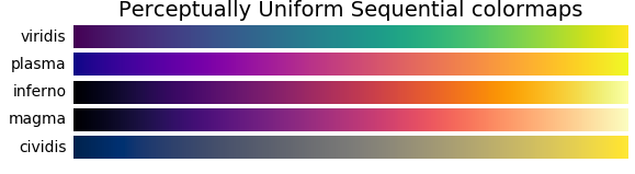
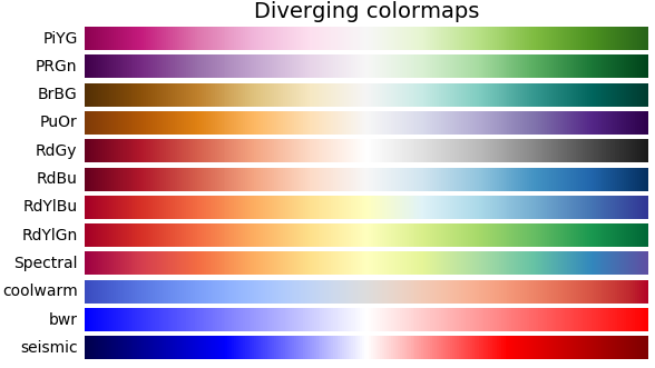
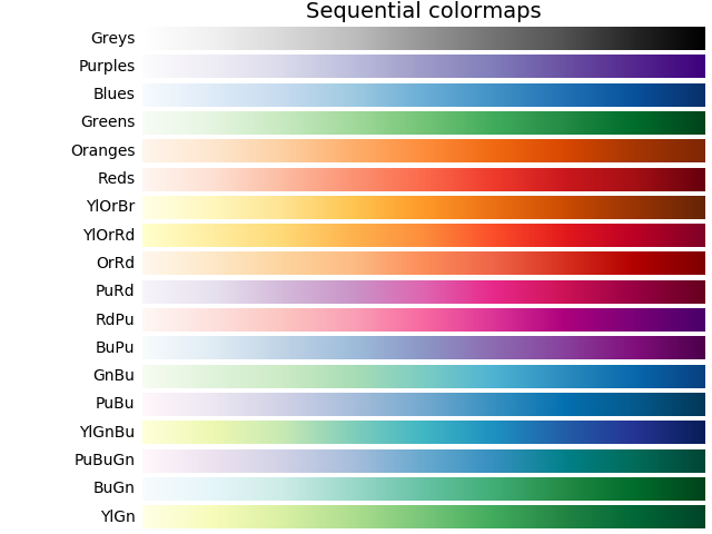
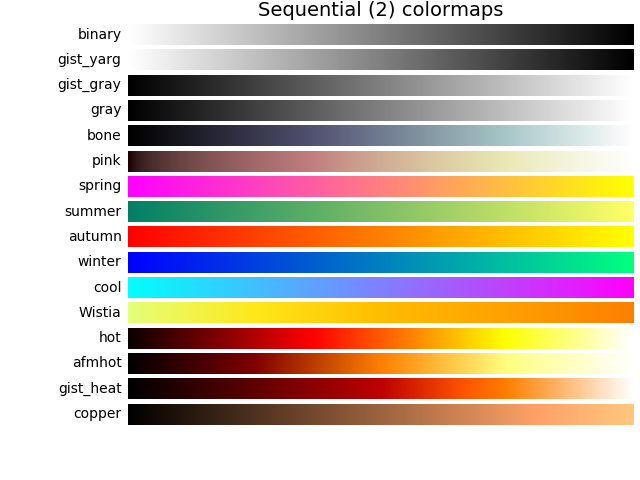
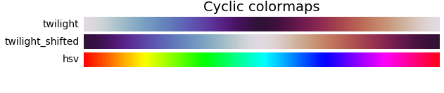
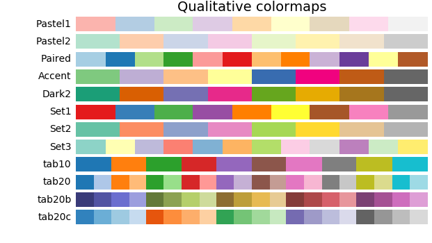
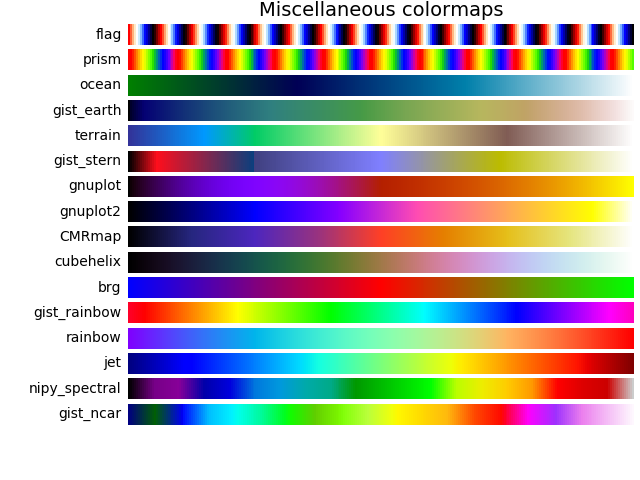
Palettes for cmap

There are 164 different palettes. Check out CMAP class and its autocompletion

idxs = [0, 3]
batch = get_batch(dls.train.dataset, idxs)

RdBu_r

show_cam(batch, model, layer=5, i2o=i2o, cmap=CMAP.RdBu_r)

viridis

show_cam(batch, model, layer=5, i2o=i2o, cmap=CMAP.viridis)

gist_gray_r

show_cam(batch, model, layer=5, i2o=i2o, cmap=CMAP.gist_gray_r)

Using different line styles

line styles :[ 'solid' | 'dashed' | 'dashdot' | 'dotted' ]

Line Style : solid - By default

show_cam(batch, model, layer=5, i2o=i2o, linewidth=2, linestyles='solid')

Line Style : dashed

show_cam(batch, model, layer=5, i2o=i2o, linewidth=2, linestyles='dashed')

Line Style : dashdot

# Gun - CAM - max
show_cam(batch, model, layer=5, i2o=i2o, linewidth=2, linestyles='dashdot')

Line Style : dotted

# Gun - CAM - max
show_cam(batch, model, layer=5, i2o=i2o, linewidth=2, linestyles='dotted')

How to use your customized CAM function

The user can create their own CAM function. Check out how both cam_acts and grad_acts_cam are define here above. Here below, as an illustration, we create a partial function that used cam_acts function

#Example using a partial
cam_acts_1 = partial(cam_acts, force_scale=False, scale_range=(0,2))
cam_acts_1.name = r'cam_acts_1'
show_cam(batch, model, layer=5, i2o=i2o, func_cam=cam_acts_1)
# Using different cmap
# **cmap possible values are: **

cmap_list = ['Accent', 'Accent_r', 'Blues', 'Blues_r', 'BrBG', 'BrBG_r', 'BuGn', 'BuGn_r', 'BuPu', 'BuPu_r', 'CMRmap', 'CMRmap_r', 'Dark2', 'Dark2_r', 'GnBu', 'GnBu_r', 'Greens', 'Greens_r', 'Greys', 'Greys_r', 'OrRd', 'OrRd_r', 'Oranges', 'Oranges_r', 'PRGn', 'PRGn_r', 'Paired', 'Paired_r', 'Pastel1', 'Pastel1_r', 'Pastel2', 'Pastel2_r', 'PiYG', 'PiYG_r', 'PuBu', 'PuBuGn', 'PuBuGn_r', 'PuBu_r', 'PuOr', 'PuOr_r', 'PuRd', 'PuRd_r', 'Purples', 'Purples_r', 'RdBu', 'RdBu_r', 'RdGy', 'RdGy_r', 'RdPu', 'RdPu_r', 'RdYlBu', 'RdYlBu_r', 'RdYlGn', 'RdYlGn_r', 'Reds', 'Reds_r', 'Set1', 'Set1_r', 'Set2', 'Set2_r', 'Set3', 'Set3_r', 'Spectral', 'Spectral_r', 'Wistia', 'Wistia_r', 'YlGn', 'YlGnBu', 'YlGnBu_r', 'YlGn_r', 'YlOrBr', 'YlOrBr_r', 'YlOrRd', 'YlOrRd_r', 'afmhot', 'afmhot_r', 'autumn', 'autumn_r', 'binary', 'binary_r', 'bone', 'bone_r', 'brg', 'brg_r', 'bwr', 'bwr_r', 'cividis', 'cividis_r', 'cool', 'cool_r', 'coolwarm', 'coolwarm_r', 'copper', 'copper_r', 'cubehelix', 'cubehelix_r', 'flag', 'flag_r', 'gist_earth', 'gist_earth_r', 'gist_gray', 'gist_gray_r', 'gist_heat', 'gist_heat_r', 'gist_ncar', 'gist_ncar_r', 'gist_rainbow', 'gist_rainbow_r', 'gist_stern', 'gist_stern_r', 'gist_yarg', 'gist_yarg_r', 'gnuplot', 'gnuplot2', 'gnuplot2_r', 'gnuplot_r', 'gray', 'gray_r', 'hot', 'hot_r', 'hsv', 'hsv_r', 'inferno', 'inferno_r', 'jet', 'jet_r', 'magma', 'magma_r', 'nipy_spectral', 'nipy_spectral_r', 'ocean', 'ocean_r', 'pink', 'pink_r', 'plasma', 'plasma_r', 'prism', 'prism_r', 'rainbow', 'rainbow_r', 'seismic', 'seismic_r', 'spring', 'spring_r', 'summer', 'summer_r', 'tab10', 'tab10_r', 'tab20', 'tab20_r', 'tab20b', 'tab20b_r', 'tab20c', 'tab20c_r', 'terrain', 'terrain_r', 'twilight', 'twilight_r', 'twilight_shifted', 'twilight_shifted_r', 'viridis', 'viridis_r', 'winter', 'winter_r']

cmaps = [f'{n} = \'{n}\'' for n in cmap_list]
# cmaps

Palettes