# Run this cell to install the latest version of fastai2 shared on github
!pip install git+https://github.com/fastai/fastai2.git

# Run this cell to install the latest version of fastcore shared on github
!pip install git+https://github.com/fastai/fastcore.git

# Run this cell to install the latest version of timeseries shared on github
!pip install git+https://github.com/ai-fast-track/timeseries.git

%reload_ext autoreload
%autoreload 2
%matplotlib inline

from fastai2.basics import *

from timeseries.all import *

Class Activation Map (CAM) and Grafient-CAM (GRAD-CAM) Tutorial

Both CAM and GRAD-CAM allow producing ‘visual explanations’ on how a Convolutional Neural Network (CNN) model based its classification and therefore help interpreting the obtained results. The InceptionTime model is used as an illustration in this notebook.

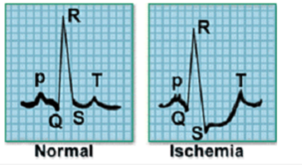
ECG Dataset

This dataset was formatted by R. Olszewski as part of his thesis “Generalized feature extraction for structural pattern recognition in time-series data,” at Carnegie Mellon University, 2001. Each series traces the electrical activity recorded during one heartbeat. The two classes are a normal heartbeat and a Myocardial Infarction. Cardiac ischemia refers to lack of blood flow and oxygen to the heart muscle. If ischemia is severe or lasts too long, it can cause a heart attack (myocardial infarction) and can lead to heart tissue death.

Training a model

# You can choose any of univariate dataset listed the `data.py` file
path = unzip_data(URLs_TS.UNI_ECG200)

dsname =  'ECG200' # 'GunPoint'
fname_train = f'{dsname}_TRAIN.arff'
fname_test = f'{dsname}_TEST.arff'
fnames = [path/fname_train, path/fname_test]
fnames

[Path('/home/farid/.fastai/data/ECG200/ECG200_TRAIN.arff'),
 Path('/home/farid/.fastai/data/ECG200/ECG200_TEST.arff')]

# num_workers=0 is for Windows platform
dls = TSDataLoaders.from_files(bs=64,fnames=fnames, num_workers=0) 

dls.show_batch(chs=range(0,12,3))

learn = ts_learner(dls)
learn.fit_one_cycle(25, lr_max=1e-3) 

epoch	train_loss	valid_loss	accuracy	time
0	1.477478	0.692645	0.575000	00:01
1	1.418432	0.693228	0.300000	00:01
2	1.247476	0.694551	0.425000	00:01
3	1.169967	0.695732	0.425000	00:01
4	1.026473	0.697049	0.425000	00:01
5	0.921037	0.700040	0.425000	00:01
6	0.831905	0.702114	0.425000	00:01
7	0.760788	0.703392	0.425000	00:01
8	0.701200	0.708715	0.425000	00:01
9	0.652415	0.708759	0.425000	00:01
10	0.610008	0.705038	0.425000	00:01
11	0.573161	0.698569	0.425000	00:01
12	0.541027	0.683905	0.425000	00:01
13	0.512720	0.661773	0.500000	00:01
14	0.487877	0.634480	0.575000	00:01
15	0.466010	0.602281	0.750000	00:01
16	0.446488	0.561948	0.850000	00:01
17	0.428792	0.512738	0.950000	00:01
18	0.413006	0.466702	0.975000	00:01
19	0.398709	0.428802	0.950000	00:01
20	0.385927	0.400146	0.925000	00:01
21	0.374558	0.374902	0.925000	00:01
22	0.364030	0.356121	0.925000	00:01
23	0.354384	0.340358	0.925000	00:01
24	0.345539	0.328972	0.925000	00:01

learn.show_results()

model = learn.model.eval()

model[5]

SequentialEx(
  (layers): ModuleList(
    (0): InceptionModule(
      (bottleneck): Conv1d(128, 32, kernel_size=(1,), stride=(1,))
      (convs): ModuleList(
        (0): Conv1d(32, 32, kernel_size=(39,), stride=(1,), padding=(19,), bias=False)
        (1): Conv1d(32, 32, kernel_size=(19,), stride=(1,), padding=(9,), bias=False)
        (2): Conv1d(32, 32, kernel_size=(9,), stride=(1,), padding=(4,), bias=False)
      )
      (maxpool_bottleneck): Sequential(
        (0): MaxPool1d(kernel_size=3, stride=1, padding=1, dilation=1, ceil_mode=False)
        (1): Conv1d(128, 32, kernel_size=(1,), stride=(1,), bias=False)
      )
      (bn_relu): Sequential(
        (0): BatchNorm1d(128, eps=1e-05, momentum=0.1, affine=True, track_running_stats=True)
        (1): ReLU()
      )
    )
    (1): Shortcut(
      (act_fn): ReLU(inplace=True)
      (conv): Conv1d(128, 128, kernel_size=(1,), stride=(1,), bias=False)
      (bn): BatchNorm1d(128, eps=1e-05, momentum=0.1, affine=True, track_running_stats=True)
    )
  )
)

dls.vocab

(#2) ['-1','1']

Decoding class labels

# i2o() function
# Converting CategoryTensor label into the human-readable label
lbl_dict = dict([
    (0, 'Normal'),   
    (1, 'Myocardial Infarction')]
)
def i2o(y):
    return lbl_dict.__getitem__(y.data.item())
    # return lbl_dict.__getitem__(int(dls.tfms[1][1].decodes(y)))

Creating a customized batch : list of 2 items

Note: This is not a batch in literal sense as used using DataLoader.one_batch() method. It just a list of some dataset items

- batch[0]: corresponds to Normal ECG

• batch[1]: corresponds to Myocardial Infarction

idxs = [0,2]
batch = get_batch(dls.train.dataset, idxs)

Plotting CAM for several dataset items in one shared figure

Example:the function expects a list of items and plots CAM for the provided items list.

Class Activation Map (CAM)

This option calculates the activations values at the selected layer.By default the activations curves are plotted in one single figure.

func_cam=cam_acts : activation function name (activation values at the chosen model layer). It is the default value

The figure title [Myocardial Infarction - Normal] - CAM - mean should be read as follow:

• Myocardial Infarction : class of the first curve
• Normal : class of the second curve
• CAM : activation function name (activation values at the chosen model layer)
• mean : type of reduction (read the explanation below: 4 types of reductions)

show_cam(batch, model, layer=5, i2o=i2o, func_cam=cam_acts) # default:  func_cam=cam_acts, multi_fig=False, figsize=(6,4)

Plot each time series curve in a separate figure

Using CAM and CMAP.seismic palette

show_cam(batch, model, layer=5, i2o=i2o, multi_fig=True, cmap=CMAP.seismic) # default: func_cam=cam_acts, figsize=(13,4)

Using GRAD-CAM and CMAP.seismic palette

Notice the difference in activations values between CAM and GRAD-CAM

show_cam(batch, model, layer=5, i2o=i2o, func_cam=grad_cam_acts, multi_fig=True, cmap=CMAP.seismic) 

Superimposed curves give another insight in comparing the 2 time series

show_cam(batch, model, layer=5, i2o=i2o, func_cam=grad_cam_acts, cmap=CMAP.seismic)

Plotting scattered lines

show_cam(batch, model, layer=5, i2o=i2o, linewidth=2, scatter=True, cmap=CMAP.hot_r)

Plotting CAM for a batch of items

We can also feed the show_cam() a full batch return straight from DataLoaders `one_batch() method as shown here below

Creating a batch of 5 items

dls.train = dls.train.new(bs=5)
batch = dls.train.one_batch()
# batch

show_cam(batch, model, layer=5, i2o=i2o, cmap=CMAP.viridis)

show_cam(batch, model, layer=5, i2o=i2o, cmap=CMAP.viridis, multi_fig=True, figsize=(18, 8), linestyles='dotted')

show_cam(batch, model, layer=5, i2o=i2o, func_cam=grad_cam_acts, multi_fig=True, figsize=(18, 8))

Plotting CAM for a single dataset item

We can also feed the show_cam() a single item

There are also 164 different palettes. Check out CMAP class and its autocompletion

line styles :'solid' | 'dashed' | 'dashdot' | 'dotted'

idxs = [0]
batch = get_batch(dls.train.dataset, idxs)

show_cam(batch, model, layer=5, i2o=i2o, cmap='rainbow', linewidth=2, linestyles='dotted')