# Run this cell to install the latest version of fastai2 shared on github
!pip install git+https://github.com/fastai/fastai2.git

# Run this cell to install the latest version of fastcore shared on github
!pip install git+https://github.com/fastai/fastcore.git

# Run this cell to install the latest version of timeseries shared on github
!pip install git+https://github.com/ai-fast-track/timeseries.git

%reload_ext autoreload
%autoreload 2
%matplotlib inline

from fastai2.basics import *

from timeseries.all import *

Class Activation Map (CAM) and Grafient-CAM (GRAD-CAM) Tutorial

Both CAM and GRAD-CAM allow producing ‘visual explanations’ on how a Convolutional Neural Network (CNN) model based its classification and therefore help interpreting the obtained results. The InceptionTime model is used as an illustration in this notebook.

GunPoint Dataset

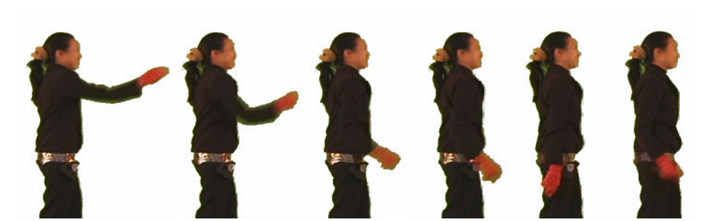
This dataset involves one female actor and one male actor making a motion with their hand. The two classes are:Gun-Draw and Point:For Gun-Draw the actors have their hands by their sides. They draw a replicate gun from a hip-mounted holster, point it at a target for approximately one second, then return the gun to the holster, and their hands to their sides. For Point the actors have their gun by their sides. They point with their index fingers to a target for approximately one second, and then return their hands to their sides. For both classes, we tracked the centroid of the actor's right hands in both X- and Y-axes, which appear to be highly correlated. The data in the archive is just the X-axis.

Training a model

# You can choose any of univariate dataset listed the `data.py` file
path = unzip_data(URLs_TS.UNI_GUN_POINT)

dsname =  'GunPoint'
fname_train = f'{dsname}_TRAIN.arff'
fname_test = f'{dsname}_TEST.arff'
fnames = [path/fname_train, path/fname_test]
fnames

[Path('C:/Users/fh/.fastai/data/GunPoint/GunPoint_TRAIN.arff'),
 Path('C:/Users/fh/.fastai/data/GunPoint/GunPoint_TEST.arff')]

# num_workers=0 is for Windows platform
dls = TSDataLoaders.from_files(bs=64,fnames=fnames, num_workers=0) 

dls.show_batch(max_n=9)

learn = ts_learner(dls)
learn.fit_one_cycle(25, lr_max=1e-3) 

epoch	train_loss	valid_loss	accuracy	time
0	1.314982	0.692901	0.575000	00:08
1	1.291740	0.693081	0.550000	00:00
2	1.171116	0.694189	0.425000	00:00
3	1.108719	0.695350	0.425000	00:00
4	0.972143	0.696890	0.425000	00:00
5	0.864975	0.700227	0.425000	00:00
6	0.778819	0.703110	0.425000	00:00
7	0.703747	0.706291	0.425000	00:00
8	0.641936	0.710956	0.425000	00:00
9	0.592867	0.714422	0.425000	00:00
10	0.551703	0.718103	0.425000	00:00
11	0.517152	0.724617	0.425000	00:00
12	0.487694	0.720280	0.425000	00:00
13	0.462060	0.707406	0.425000	00:00
14	0.439792	0.693197	0.425000	00:00
15	0.420413	0.656317	0.425000	00:00
16	0.403305	0.612189	0.475000	00:00
17	0.388097	0.571316	0.675000	00:00
18	0.374597	0.524806	0.850000	00:00
19	0.362410	0.476796	1.000000	00:00
20	0.351393	0.433147	1.000000	00:00
21	0.341482	0.393019	1.000000	00:00
22	0.332415	0.358370	1.000000	00:00
23	0.324265	0.329521	1.000000	00:00
24	0.316777	0.306814	1.000000	00:00

learn.show_results()

model = learn.model.eval()

model[5]

SequentialEx(
  (layers): ModuleList(
    (0): InceptionModule(
      (bottleneck): Conv1d(128, 32, kernel_size=(1,), stride=(1,))
      (convs): ModuleList(
        (0): Conv1d(32, 32, kernel_size=(39,), stride=(1,), padding=(19,), bias=False)
        (1): Conv1d(32, 32, kernel_size=(19,), stride=(1,), padding=(9,), bias=False)
        (2): Conv1d(32, 32, kernel_size=(9,), stride=(1,), padding=(4,), bias=False)
      )
      (maxpool_bottleneck): Sequential(
        (0): MaxPool1d(kernel_size=3, stride=1, padding=1, dilation=1, ceil_mode=False)
        (1): Conv1d(128, 32, kernel_size=(1,), stride=(1,), bias=False)
      )
      (bn_relu): Sequential(
        (0): BatchNorm1d(128, eps=1e-05, momentum=0.1, affine=True, track_running_stats=True)
        (1): ReLU()
      )
    )
    (1): Shortcut(
      (act_fn): ReLU(inplace=True)
      (conv): Conv1d(128, 128, kernel_size=(1,), stride=(1,), bias=False)
      (bn): BatchNorm1d(128, eps=1e-05, momentum=0.1, affine=True, track_running_stats=True)
    )
  )
)

Decoding class labels

# i2o() function
# Converting CategoryTensor label into the human-readable label
lbl_dict = dict([
    (0, 'Gun'),   
    (1, 'Point')]
)
def i2o(y):
    return lbl_dict.__getitem__(y.data.item())
    # return lbl_dict.__getitem__(int(dls.tfms[1][1].decodes(y)))

Creating a customized batch : list of 2 items

Note: This is not a batch in literal sense as used using DataLoader.one_batch() method. It just a list of some dataset items

- batch[0]: corresponds to Gun gesture

• batch[1]: corresponds to Point gesture

idxs = [0,3]
batch = get_batch(dls.train.dataset, idxs)
# len(batch), type(batch)

Plotting CAM for several dataset items in one shared figure

Example:the function expects a list of items and plots CAM for the provided items list.

Class Activation Map (CAM)

This option calculates the activations values at the selected layer.By default the activations curves are plotted in one single figure.

func_cam=cam_acts : activation function name (activation values at the chosen model layer). It is the default value

The figure title [Gun - Point] - CAM - mean should be read as follow:

• Gun : class of the first curve
• Point : class of the second curve
• CAM : activation function name (activation values at the chosen model layer)
• mean : type of reduction (read the explanation below: 4 types of reductions)

show_cam(batch, model, layer=5, i2o=i2o, func_cam=grad_cam_acts) # default:  func_cam=cam_acts, multi_fig=False, figsize=(6,4)

Plot each time series curve in a separate figure

show_cam(batch, model, layer=5, i2o=i2o, multi_fig=True) # default: func_cam=cam_acts, figsize=(13,4)

Gradiant Class Activation Map (GRAD-CAM)

This option calculates the gradient activations values at the selected layer.

We supply the argument func_cam=grad_cam_acts to calculate the Gradient-Class Activation Map (GRAD-CAM)

Note: another palette is also used in this example: cmap=CMAP.seismic

show_cam(batch, model, layer=5, i2o=i2o, func_cam=cam_acts, reduction='max', cmap=CMAP.seismic)

Using RAW activation values: force_scale=False (Non-scaled values)

By default, both func_cam=grad_cam_acts (GRAD-CAM) and reduction=mean are used In this example, we are plotting the raw activation values (by default GRAD-CAM). Notice the values on the cmap color palette.

We can supply a user-defined func_cam. See here below an example with a custom defined function cam_acts_1

Pay attention to the scale values. Instead of being between [0..1], they are between th min and the max of the activation raw values

show_cam(batch, model, layer=5, i2o=i2o, func_cam=grad_cam_acts , force_scale=False, cmap='seismic')

4 types of reduction

When raw activities are caluculated, we obtain a tensor of [128, 150]. 128 corresponds to the number of channels. Whereas 150 represents the data points. Since the original time series is a [1, 128] tensor (univariate time series), we need to reduce the [128, 150] tensor to [1, 150]. Therefore, we have several types of reductions.

show_cam() offers 4 types of reductions:

• mean (default)
• median
• max
• mean_max (average of mean and max values)

Using reduction='max'

mean is the default reduction. Here below, we use max reduction

show_cam(batch, model, layer=5, i2o=i2o, func_cam=grad_cam_acts, reduction='mean_max', cmap=CMAP.seismic)

Plotting scattered lines

show_cam(batch, model, layer=5, i2o=i2o, linewidth=2, scatter=True, cmap=CMAP.hot_r)

Plotting CAM for a batch of items

We can also feed the show_cam() a full batch return straight from DataLoaders `one_batch() method as shown here below

Creating a batch of 5 items

dls.train = dls.train.new(bs=5)
batch = dls.train.one_batch()

show_cam(batch, model, layer=5, i2o=i2o, cmap=CMAP.viridis)

show_cam(batch, model, layer=5, i2o=i2o, cmap='viridis', multi_fig=True, figsize=(18, 8), linestyles='dotted')

Plotting CAM for a single dataset item

We can also feed the show_cam() a single item

idxs = [0]
batch = get_batch(dls.train.dataset, idxs)

show_cam(batch, model, layer=5, i2o=i2o, cmap='rainbow')

Palette (cmap), Line width, and Line Styles

There are 164 different palettes. Check out CMAP class and its autocompletion

line styles :'solid' | 'dashed' | 'dashdot' | 'dotted'

# reload the batch with 2 items used earlier
idxs = [0, 3]
batch = get_batch(dls.train.dataset, idxs)

show_cam(batch, model, layer=5, i2o=i2o, cmap='RdBu_r', linewidth=2, linestyles='dotted')

show_cam(batch, model, layer=5, i2o=i2o, cmap='gist_gray_r')