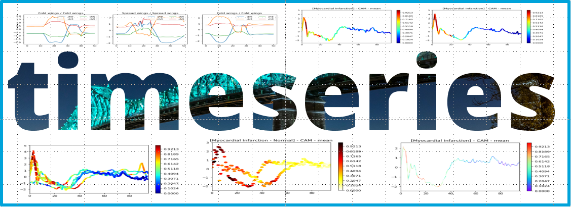
Time Series Classification Using Deep Learning - Part 1
A gentle introduction to time series classification using state of the art neural network architecture.
- Objectives:
- Introduction
- Time Series Short Introduction
- Time Series Analysis
- Toy Data
- What is the goal of the NATOPS time series classification?
- End-to-End Training
- Code Walk Through
- Conclusion
In this article, I will introduce you to a new package called timeseries for fastai2 that I lately developed. The timeseries package allows you to train a Neural Network (NN) model in order to classify both univariate and multivariate time series using the powerful fastai2 library and achieve State Of The Art (SOTA) results.
Objectives:
The key objectives of this series of articles are:
-
Introduce you to time series classification using Deep Learning,
-
Show you a step by step how this package was built using fastai2 library,
-
Introduce you to some key concepts of the fastai2 library such as Datasets, DataLoaders, DataBlock, Transform, etc.
Introduction
Unlike Computer Vision (CV), Time Series (TS) analysis is not the hottest topic in the Artificial Intelligence (AI)/DL eco-system. Lately, CV starts to lose a bit of its luster because of the amount of controversies around facial detection abusive applications among other reasons. As a potential positive consequence, we hope more attention will be geared towards TS analysis opening the door to more innovation in the TS field.
Another positive aspect of using DL in the TS field is the fact that training a NN TS model uses far less both CPU and GPU resources. As a matter of fact, it uses a fraction of the compute resources in comparison to those needed to train NN models in both CV and NLP.
Compared to both CV and Natural Language Processing (NLP), TS is still in its infancy in terms of DL innovations. This offers the opportunity to talented people to step in this domain and to start innovating and creating new models that are specifically designed to time series. Those new models could be built from the ground or inspired by some well established NN models such as ResNet in CV, and LSTM in NLP.
fastai2 could play a significant role in developing this field thanks to its unified APIs that already spans several domains such as Vison, NLP, and Tabular, on one hand, and to its level of granularity in terms of APIs depth (High, Mid, and Low Levels APIs), on the other hand.
By using fastai2, not only, this will accelerate the development of new libraries but it will also offer a fast learning curve for users exploring those new TS libraries: in other word, we can leverage the transfer learning between different modules that constitutes the fastai2 library.
Before diving in the core subject, let's define what a time series is.
Time Series Short Introduction
A time series is a simple set of data point stored in a chronological order (time stamps). Time series can be found in virtually all domains and can be divided into 2 types:
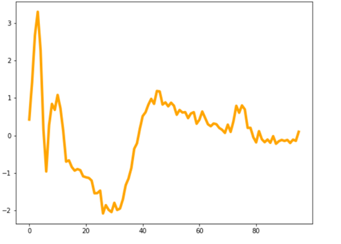
• Univariate time series: Representing a single wave. The example, here below, shows an ECG recording extracted from the ECG200 dataset. An analysis using that dataset is shown in the End-to-End Training section.
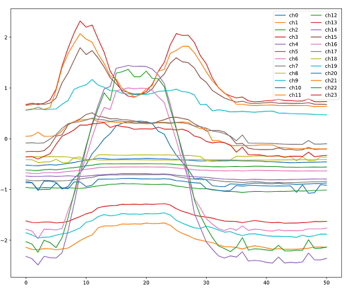
• Multivariate time series: Representing a set of related waves such as NATOPS recording which represent sensors recordings at different locations: hands, elbows, wrists and thumbs. For more details, check out the Toy Data section here below.
Time Series Analysis
Time series analysis is becoming increasingly important because of the easy access and the wide spread of time series generation tool such as mobile devices, internet of things, logging and monitoring data generated in virtually all the industries, etc. What will become even more crucial is the design of end-to-end tools capable of analyzing such a gigantic amount of data. Deep Learning will play a key role in providing such tools.
Time series analysis aims to extract meaningful information that allow the user to get actionable insights. It can be divided into 3 main categories:
- Time Series Classification (TSC): We present a time series to a Neural Network (NN) model, and the latter predicts its label (class). This article will focus on this category
- Time Series Regression (TSR): This is quite similar to TSC, and share the same data processing. It can be seen as TSC special case where the number of labels (classes) is reduced to 1, and represented by a float instead of an integer (category)
- Time Series Forecasting (TSF): it consists in predicting the future values (or range of values) of a time series (e.g. temperature, sales, stock price, etc.) based on previously observed values
The timeseries package presented in this article covers both time series classification and regression.
Many big companies and startups are heavily investing in developing both AI-enabled processors and micro-controllers for AI in edgepoint Applications.
Nowadays, the edge AI portion of a smartphone System-on-Chip (SoC) represents only about 5% of the total area and about US$3.50 of the total cost, and would use about 95% less power than the whole SoC does. This stressed out how affordable the AI chips already are.
The wide spread of both AI chips and artificial intelligence of things (AIoT) will make NN model training and/or inference at edgepoints a reality. AI inference on the edgepoint device is very attractive because it decreases latency, saves bandwidth, helps privacy, and saves power associated with RF transmission of data to the cloud.
Furthermore, the ability to collect, interpret, and immediately act on vast amounts of data is critical for many of the data-heavy applications.
As a consequence, this will likely drive significant changes for consumers and enterprises applications. Smart machines powered by AI chips will have a huge impact on a wide variety of industries such as manufacturing, logistics, agriculture, energy, etc.
TS processing using AI/DL techniques could play a key role in implementing AI in edgepoint given the fact that TS uses far less resources such as memory and compute than both CV and NLP counterparts.
Toy Data
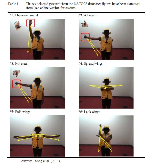
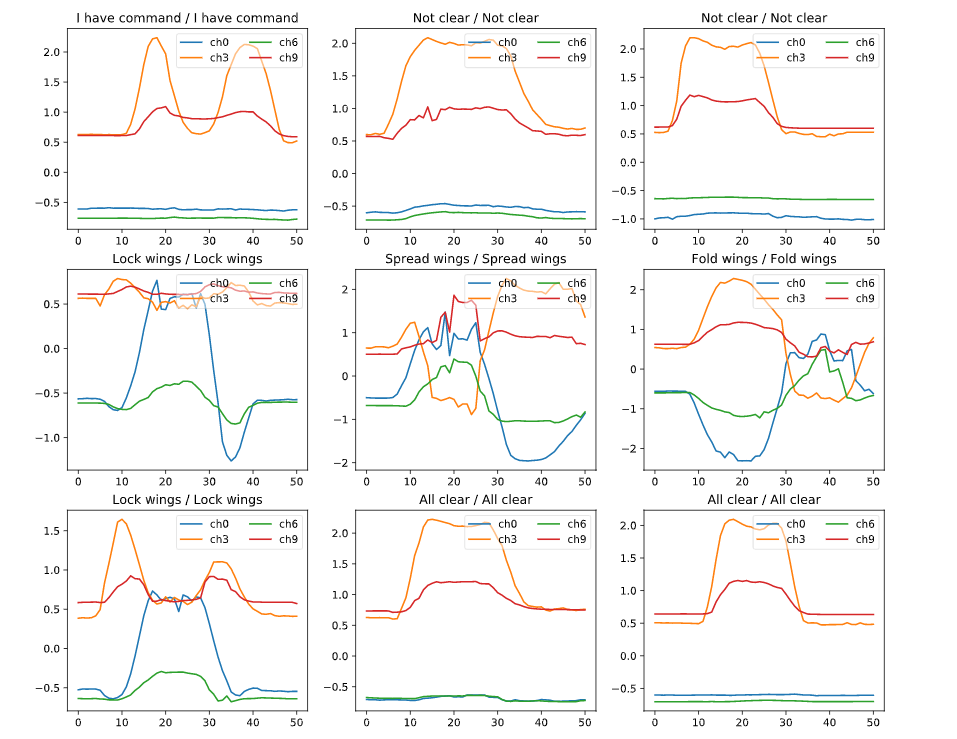
As an illustration, I will use a multivariate time series from Naval Air Training and Operating Procedures Standardization (NATOPS) dataset. The data is generated by sensors on the hands, elbows, wrists and thumbs (see figure here above). The data are the x, y, z coordinates for each of the 8 locations. For each sensor and each axis, we have a time series that represent the value of x (respectively y, and z) during the execution of a command. For instance, channel 3 (ch3) on the graph, here above, shows the Hand tip right X coordinate at different timestamps. For each gesture, we will have 24 curves corresponding to 8 sensors x 3 coordinates. The whole represents a multivariate time series.
Classes (Labels)
The dataset contains six classes representing 6 separate actions, with the following meaning: 1: I have command 2: All clear 3: Not clear 4: Spread wings 5: Fold wings 6: Lock wings
What is the goal of the NATOPS time series classification?
The NATOPS dataset contains time series recordings corresponding to different commands executed by different operators.
The goal is to train our NN model using both a training dataset and a valid dataset. After training our model and achieving a high accuracy score, we feed our model a given sensor test data without providing its class (label) (e.g. "4: Spread wings"), and our model will predict which class the sensor data correspond to (hopefully "4: Spread wings").
End-to-End Training
In this section, I will show how easy to train a NN model, and achieve some SOTA results in a record time. Before doing that, let’s introduce the timeseries package. The latter was designed to mimic the unified fastai v2 APIs used for vision, text, and tabular in order to ease its use among users familiar with the fastai2 APIs. As a consequence, those who already used fastai2 vision module will feel familiar with the timeseries APIs. Timeseries package uses Datasets, DataBlock, and a new TSDataLoaders and a new TensorTS classes. It has the following mapping with fastai2 vision module:
TensorImage <---> TensorTS
Conv2D <---> Conv1D
The timeseries package also references 128 Univariate and 30 Multivariate time series datasets. Using URLs_TS class (similar to fastai URLs class) you might play with one of those 158 datasets.
Similarly to fastai vision examples, we can train any time series dataset end-to-end with 4 lines of code. In the example shown, here below, we use TSDataLoaders and the multivariate NATOPS dataset.
path = unzip_data(URLs_TS.NATOPS)
dls = TSDataLoaders.from_files(bs=32,fnames=[path/'NATOPS_TRAIN.arff', path/'NATOPS_TEST.arff'], batch_tfms=[Normalize()])
learn = ts_learner(dls)
learn.fit_one_cycle(25, lr_max=1e-3)
Using a SOTA NN model called InceptionTime (published in September 2019), and the default fastai2 settings, we can achieve around 98,5% accuracy in only 20 epochs. The following figure shows some of the predictions results (Predicted/True classes):
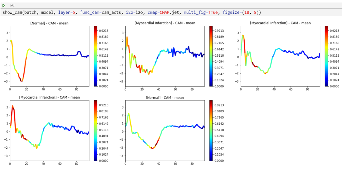
The package also features Class Activation Map (CAM) for time series. CAM is used to help interpreting the results of our NN model decision. The package offers both CAM and GRAD-CAM as well as user-defined CAM. The cam_tutorial_ECG200.ipynb notebook illustrates a simple example of the univariate ECG200 dataset classification task (Normal Heartbeat vs. Myocardial Infarction). Like in vision, the colors represent the activation values at a given layer (in this example it is located before the FC layer (last layer)). Notice how the Myocardial Infarction plots (2nd, 3rd, and 4th) share similar activation zones that are quite different from those corresponding to Normal Heartbeat plots (1st and 5th). This kind of representation eases the interpretation of the results obtained using a given NN model (InceptionTime, in this case).
Code Walk Through
let’s decipher, line by line, the 4 lines of code shown here above:
-
Line 1: Downloading Data
path = unzip_data(URLs_TS.NATOPS)Downloading a dataset (NATOPS dataset precisely) hosted at the Time Series Classification Repository website, unzipping the dataset, and saving it a separate folder under the local ./fastai/data folder.
-
Line 2: Creating Datasets and DataLoaders Objects
dls = TSDataLoaders.from_files(bs=32,fnames=[path/'NATOPS_TRAIN.arff', path/'NATOPS_TEST.arff'], batch_tfms=[Normalize()])-
Creating a 2 Dataset objects containing a train dataset, and a valid dataset.
-
Creating 2 DataLoader objects that allows us to create mini-batches for both training and valid datasets.
-
-
Line 3: Creating a Learner Object
learn = ts_learner(dls)We create a learner where we basically do the following:
-
Create an NN model, InceptionTime in our case.
-
Create a Learner object using some state-of-the-art techniques found in the fastai2 library such as the Ranger optimizer, callbacks, etc.
-
-
Line 4: Training Model
learn.fit_one_cycle(25, lr_max=1e-3)We train our model using one the fastai magic ingredient being the fast converging training algorithm called fit_one_cycle(). Running the last line, we achieve accuracy higher than 98% in less than 20 epochs.
Admittedly, the 4 lines shown here above can be a bit cryptic for someone how is new to the fastai2 library. Those lines show how to train a model using the fastai2 high level API. At that level, many settings are set by default in order to avoid overwhelming new users by exposing too many parameters that are difficult to grasp at the beginning of their learning journey. As shown here above, using fastai2 default settings we are very often capable of reaching SOTA results in fewer epochs.
As a very versatile API covering a large range of use-cases, fastai2 offers 3 levels of APIs: High level, Mid Level, and Low Level. Depending on both use-cases and user's fastai2 proficiency, one might choose one or the other level.
In the next article, I will take that opportunity to start building the timeseries module using the Mid Level APIs. I chose that level because both fastai version 1 and/or Pytorch users will feel in familiar territories. We will leverage the new fastai2 Datasets and DataLoaders classes, and show how both versatile and powerful are.
Conclusion
I hope this first article convey you into trying the timeseries package. You might also check out its documentation. All the notebooks are self-contained, and documented. You will be able to directly run them in Google Colab.
If you give it a try and found it interesting/helpful, please let others know it by staring it on GitHub, and share it with your friends and colleagues who might be interested in this topic.
As a new Twitter user, I would like to kindly ask you to follow me @ai_fast_track. I will post there the sequel of this blog post.
I also intend to post on Twitter, on regular basis, Tips & Tricks about fastai(2) and Deep Learning in general. Stay Tuned, and Stay Safe!